Polina Vytnova

My github contains raw code (in Fortran and C) used to study some dynamical systems I am interested in.
The continued fraction is an alternative way to represent a real number as a limit of a sequence of rational numbers. Recall that for a real number α its continued fraction is an expression of the form
| α = |
|
= a0+1/(a1+1/(a2+1/(a3+...))) = |
[a0; a1, a2, a3, ... ] |
||||||||||||
| 1 |
| x |
| [ | 1 | ] |
| x |
T: [0;a1,a2,a3...] ↦ [0;a2,a3,a4...]
It is therefore not invertible, but has infinitely many inverse branches Tj : x ↦| 1 |
| x + j |
Tj : [0;a1,a2,a3...] ↦ [0;j,a1,a2,a3...]
We may pick a pair of integers, say, 1 and 2 and consider an iterated function scheme of two inverse branches T1,T2. Then for any α∈[0,1] = [0;a1,a2,a3...] and for any sequence {jn} of 1s and 2s the imagesTjn...Tj3Tj2Tj1 : α= [0;a1,a2,a3...] ↦ [0;jn,...,j3,j2,j1,a1,a2,a3...]
converge to a number whose partial denominators are all either 1 or 2. The set of all such numbers has been well studied and even has a dedicated notation.C2 = {x ∈ (0,1) | x = [0; a1, a2, a3, ... ], where aj = 1 or aj = 2 for all indices j }.
It is a nonlinear Cantor set and it has a complex fractal structure. More generally, the sets which arise as limit sets of iterated function schemes of (a finite number of) the inverse branches Tj are called Gauss—Cantor sets. The Hausdorff dimension of C2 has now been computed to very high accuracy and we give 200 digits of it in Section 4.1.2 of our paper. For practical applications it is useful to know thatdimH C2 = 0.53128... > 0.5.
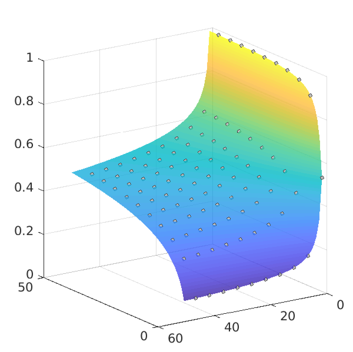
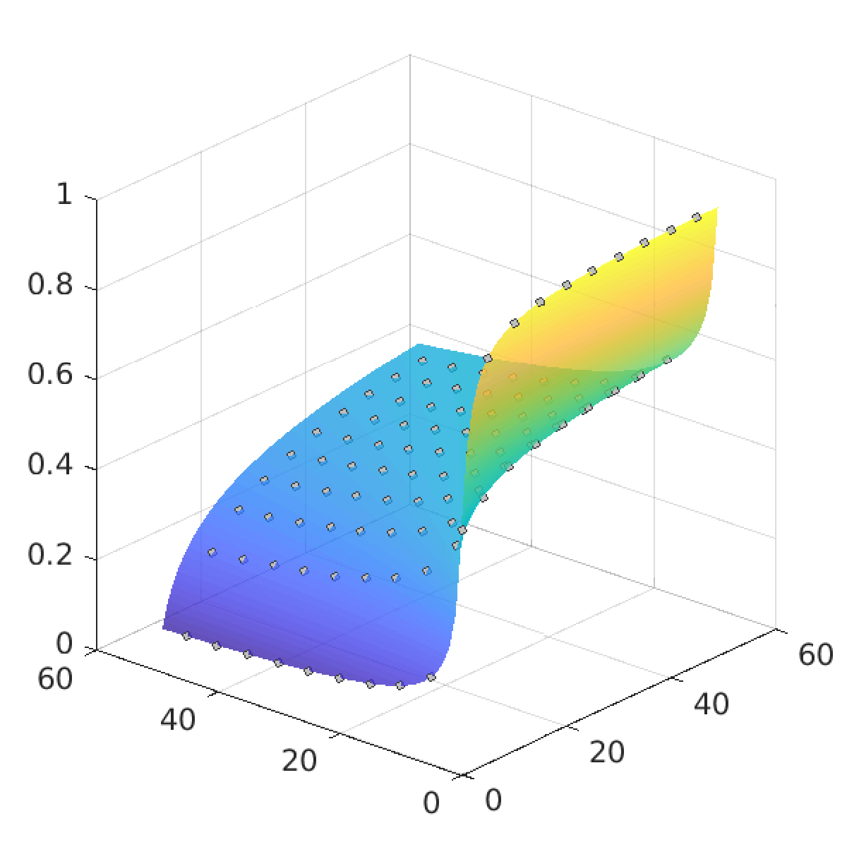
Figure 1 on the left depicts the dimension of a two-parameter family of setsEn,k = {x ∈ (0,1) | x = [0; a1, a2, a3, ... ], where aj ∈ {n, n+1, ... , n+k} for all indices j }
as a function of two variables d(n,k) = dimH En,k for n,k = 1, ... , 50 . The set C2 corresponds to the choices n = 1 and k = 1, so C2 = E1,1. The method we developed allows us to compute these 2500 values in just a few minutes with accuracy of 10−5. We see that for any fixed k0 the function d(n,k0) decreases rather rapidly as a function of n. For instance, in a special case k0 = 1 with only two digits n and n+1 in the expansion, we getd(2,1) = 0.3374... , d(3,1) = 0.2637... , d(50,1) = 0.0883....
On the other side of the parameter domain, when k0 = 50 we haved(1,50) = 0.9872..., d(2,50) = 0.8085..., d(50,50) = 0.4594....
Our algorithm enabled us to establish several estimates on the dimension of Gauss—Cantor sets, which are essential for the results on the density-one and modular forms of the Zaremba conjecture (pdf). Continued fractions also appear in Diophantine approximation in connection with the Markov and Lagrange spectra. The Markov spectrum first appeared in 1879–80 in work by A. A. Markov (father) on quadratic forms. Later, Perron gave an alternative definition, in terms of continued fractions. On a set of bi-infinite sequences of natural numbers, we may define a real-valued functionλ : {an} ↦ a0 + [0;a1,a2,a3...] + [0;a−1,a−2,a−3...] ∈ R.
Then the Markov number of {an} is defined as a limit of the values of λ along the trajectory of the Bernoulli shift σ : {an} ↦ {an+1} , namelym({an}) := limj→∞ λ(σj{an}).
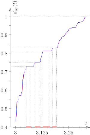
The (classical) Markov spectrum M is then defined as the set of all Markov numbers for all possible sequences of integers. It is known that (-∞,3) ∩ M is a discrete set and M ∩ (√21,+∞) is the entire ray. In the interval [3,√21] the Markov spectrum has rich fractal structure. Figure 2 on the left shows an approximation to the dimension of (-∞,t) ∩ M as a function of t. A recent result by C. G. Moreira shows that dM(t)=dimH((-∞,t) ∩ M) is a Cantor function, i.e. a continuous function which is locally constant on an open dense set. The approximation was calculated using the method we developed in our paper (joint with C. Matheus, C. G. Moreira and M. Pollicott), where we study other properties of the Markov spectrum and its closely related cousin called the Lagrange spectrum. The pink intervals show the gaps in the Markov spectrum, which are given, for instance, in the Cusick and Flahive’s textbook “Markov and Lagrange spectra” (published in 1991).PhD Thesis, University of Warwick,
under supervision of Dr. Oleg Kozlovski:
♜ Kinematic fast dynamo problem (pdf)
♜ Viva Talk Handout (pdf)
MRI Master Class project, University of Utrecht, under supervision of Prof. Yu. Kuznetsov:
♝ Accumulation of strong 1:2 resonances in generalised Hénon maps (pdf)
MSc Thesis, Independent University of Moscow, under supervision of Prof. G. Shabat:
♞ On nonarchimedean dynamical systems (pdf)